In my linear algebra course, we were handed the following rotation matrix to memorize:

I mean, sure, it does rotate a coordinate by $\theta$, but it doesn’t feel very inspired. It’s just a bunch of sines and cosines. Why does it work? If I was laying out linear algebra myself, how could I come up with this same matrix? Could I generalize it to any dimension?

I think it’s a rich question that puts to use a lot of interesting linear algebra machinery. Even then, I’ve designed this post to be approachable with limited linear algebra knowledge, hopefully—no eigenvalues or row echelon forms or any of that. I hope to show what made the orthogonal group, $O(n)$, feel a little more natural to me.

$R_\theta$?

Why $R_\theta$, in particular, describes a rotation by $\theta$ is the easiest question to answer.

Expressing $R_\theta$ as angle addition

One strategy to convince yourself would be to draw a circle with some initial vector $\vec{v}$ on its circumference. Label the vector after rotation $\vec{u}$, and draw $\theta$ in between the two. With a little line-drawing and angle-hopping, you’ll rediscover the angle addition formula.

Concretely, $\vec{v}$ can be written in “polar form” as $r\begin{bmatrix} \cos{\omega} \\ \sin{\omega} \end{bmatrix}$. $\vec{u}$ is just $\vec{v}$ rotated by $\theta$, or $r\begin{bmatrix} \cos{(\omega+\theta)} \\ \sin{(\omega+\theta)} \end{bmatrix}$. The angle addition formula you discovered geometrically will then tell you this is the same as $r\begin{bmatrix} \cos{\omega}\cos{\theta}-\sin{\omega}\sin{\theta} \\ \sin{\omega}\cos{\theta}+\cos{\omega}\sin{\theta} \end{bmatrix}$. Since the expression is linear in terms of $\cos{\omega}$ and $\sin{\omega}$, it can be expressed as: $r\begin{bmatrix} \cos{\theta} & -\sin{\theta} \\ \sin{\theta} & \cos{\theta} \end{bmatrix}\begin{bmatrix} \cos{\omega} \\ \sin{\omega} \end{bmatrix}$. Since this matrix doesn’t scale the vector’s length, this expression is the same as $\begin{bmatrix} \cos{\theta} & -\sin{\theta} \\ \sin{\theta} & \cos{\theta} \end{bmatrix}r\begin{bmatrix} \cos{\omega} \\ \sin{\omega} \end{bmatrix}$, or $\begin{bmatrix} \cos{\theta} & -\sin{\theta} \\ \sin{\theta} & \cos{\theta} \end{bmatrix}\vec{v}$. I didn’t like this solution since it’s very mechanical and not exactly enlightening.

Expressing $R_\theta$ with its basis vectors

If you’re easier to convince and prefer an explanation with more linear algebra, it’d suffice to show that:

• Our first basis vector, $\hat{\imath}$, must be $\begin{bmatrix} \cos{\theta} \\ \sin{\theta} \end{bmatrix}$, since it must rotate the vector $\begin{bmatrix} 1 \\ 0 \end{bmatrix}$ to $\begin{bmatrix} \cos{\theta} \\ \sin{\theta} \end{bmatrix}$. This makes sense—a point sitting at $(0, 1)$ at the origin should map to $(\cos{\theta}, \sin{\theta})$ after being rotated by angle $\theta$.
• Similarly, our second basis vector, $\hat{\jmath}$, must be $\begin{bmatrix} -\sin{\theta} \\ \cos{\theta} \end{bmatrix}$, since it must rotate the vector $\begin{bmatrix} 0 \\ 1 \end{bmatrix}$ to $\begin{bmatrix} \cos(\theta+\frac{\pi}{2}) \\ \sin(\theta+\frac{\pi}{2}) \end{bmatrix}$ or, after simplifying, $\begin{bmatrix} -\sin{\theta} \\ \cos{\theta} \end{bmatrix}$. This makes also sense—$\hat{\jmath}$ is $90^\circ$ ahead of $\hat{\imath}$, so it should be offset by that much to stay orthogonal after rotation.
• Since a matrix is exclusively described by its basis vectors, $R_\theta = \begin{bmatrix} \cos{\theta} & -\sin{\theta} \\ \sin{\theta} & \cos{\theta} \end{bmatrix}$.

I liked this explanation more since it utilizes an important fact about rotations: the basis vectors are always orthogonal. If the vectors weren’t orthogonal, you’d get “scaling bias” in the direction the vectors are concentrated in. This would create some form of elliptic rotation (that includes scaling), instead of the pure circular symmetry we desire in our definition of a rotation matrix. However, this fact is something you need to convince yourself of since it isn’t algebraically obvious, making this explanation lacking.

It goes without saying that there are probably many more derivations, I probably just didn’t think of them.

$O(n)$?

Let’s return to our core question—how could I have come up with rotation matrices myself? If I didn’t know anything about sines or cosines, neither explanation is useful.

Defining a rotation matrix

Okay, it might help to ask something more substantial. What makes a matrix a rotation matrix? Well, that one’s a bit silly too, since all matrices are rotation matrices to some extent. They all represent linear transformations, and linear transformations represent scaling and rotating the input, even if that rotation is zero degrees.

Well, for the purposes of our problem, what do we not want to consider a rotation matrix? For my definition, I chose any matrix that scales the input vector—i.e. modifies its length—to be a non-rotation matrix. In other words,

will be considered rotation matrices by me.

[!warning] This isn’t the correct construction of a rotation matrix.
This definition has a subtle flaw that’ll be addressed later. For now, treat it as if it is.

The rotation equations

Let’s start in $n = 2$. What does our scaling constraint say about the matrix? Let’s try to compute the norm symbolically and see.

Although this doesn’t look too interesting just yet, consider this: no matter what $x$ and $y$ are, this equation needs to hold true. That’s pretty restrictive! I’m going to call it the “norm equation”. Let’s expand and group like terms.

In order for this equation to be universally true across all values of $x$ and $y$,

Behold! The rotation equations!

Understanding rotation matrices

You might notice we have three equations for four degrees of freedom. That’s to be expected! A rotation in two dimension really is just the choice of the single angle, after all. This isn’t at all true in three dimensions though: there, we have roll, pitch, and yaw. We can generalize later.

For now, look at the equations that fell out of the norm constraint! Since there’s only a single degree of freedom, we should be able to find $a(t), b(t), c(t), d(t)$ that satisfy these equations. Finding a general form for these equations feels sort of reminiscent to solving a differential equation. If you’re willing to accept something a little shoddy, I spun up a quick and dirty SageMath script to do the algebra for me.

{x00: r1, x01: sqrt(-r1^2 + 1), x10: sqrt(-r1^2 + 1), x11: -r1}
{x00: r2, x01: -sqrt(-r2^2 + 1), x10: sqrt(-r2^2 + 1), x11: r2}
{x00: r3, x01: -sqrt(-r3^2 + 1), x10: -sqrt(-r3^2 + 1), x11: -r3}
{x00: r4, x01: sqrt(-r4^2 + 1), x10: -sqrt(-r4^2 + 1), x11: r4}
{x00: 1, x01: 0, x10: 0, x11: -1}
{x00: 1, x01: 0, x10: 0, x11: 1}
{x00: -1, x01: 0, x10: 0, x11: 1}
{x00: -1, x01: 0, x10: 0, x11: -1}
{x00: 0, x01: 1, x10: 1, x11: 0}
{x00: 0, x01: -1, x10: 1, x11: 0}
{x00: 0, x01: 1, x10: -1, x11: 0}
{x00: 0, x01: -1, x10: -1, x11: 0}

You can probably already see that $R_\theta$ satisfies this equation, but also some more familiar matrices, such as as the identity matrix, the reflection across $y = x$ (this is foreshadowing), and negate-$x$.

I think it’s important to not get lost in the algebra. We can always come back later. What are these equations saying? I can’t say for certain, but my current guess is that the equations come in two flavors: magnitude and orthogonality constraints.

Magnitude and orthogonality constraints

Magnitude constraining equations, like $a^2+c^2 = 1$, require that a basis vector, like $\begin{bmatrix} a \\ c \\ \end{bmatrix}$, have a magnitude of $1$. I’d be very confused if every basis vector didn’t have this constraint. If they didn’t, applying the transformation to a unit vector would change its length.

Next are the orthogonality constraints, the equations which require the dot product of basis vectors to be zero, such as $ab + cd = 0$. If they’re not orthogonal, the rotation they’ll trace out will be elliptic, just as we forecasted.

Both of these would make so much sense! It’s not enough for the basis vectors to simply be of length one. It’s sort of like two people balancing on a seesaw. They can’t just be equal weight, they need to apply that weight in the same place to balance.

I speculate that as we bump up the dimension, we’ll get more and more orthogonality constraints. Specifically, I think there’ll be one for every pair of vectors. As we add more algebraic terms to the norm equation, we’ll have to constrain more coefficients of pairs of variables, like $zx$ or $yz$, to zero.

Generalizing to $n$ dimensions

Okay, enough guessing. What constraints will the norm equation levy for higher dimensions?

Let’s start with a hypothetical $n$ dimensional matrix on a hypothetical input vector.

Each row of the matrix is summed, weighted by each component of the input vector, to produce each component of the output vector. So our hypothetical output vector would be:

with a constrained norm of:

Alternatively, as:

We can expand each squared summation as two summations, split them up, and swap the summation order:

Notice that these summations in terms of $j$ are redundant. They’re just doing some component-by-component operation on the $i$-th or $k$-th basis vector. For example:

So our generalized norm equation becomes:

Isn’t that incredible? Who would’ve thought the norm equation was hiding all this? This formula proves our guesses about the magnitude and orthogonality constraints. In order for the left hand side to be the same as the right hand side, the length of all basis vectors needs to be one and they all need a dot product of zero with each other. Although I’m sure someone somewhere has written this expression out before, I have saved the page in my notebook with this formula on it.

I think something that is exceptionally cool about this formula that we can now predict the number of degrees of rotational freedom in a higher dimensional space, $\mathbb{R}^n$. A matrix in $n$ dimensions has $n^2$ possible variables. Since there are $n$ magnitude constraints for $n$ basis vectors and $\binom{n}{2}$ orthogonality constraints for each pair of independent basis vectors…

Magic! $\binom{n}{2}$ degrees of rotational freedom in the $n$-th dimension!

Constructing rotation matrices

That’s neat and all, but how can I go about generating these rotation matrices? Here’s an algorithm you can try:

• Pick a basis vector. You’ll have $n - 1$ options, since you’re essentially picking any vector in space, just not its length. It’s the same as picking a point on an $n$ dimensional sphere.
• Pick the next basis vector. This time, you’ll have $n - 2$ options, since you’re picking from all vectors orthogonal to the first basis vector with length one.
• Pick the next one, which will have $n - 3$ options, since it must be orthogonal to both vectors. Continue doing so, until you have no control over the last vector you pick.

For example, in three dimensions, you’d pick the first basis vector on a sphere. You’d then pick the next basis vector off a circle on the sphere that represents all vectors orthogonal to the first. The final vector is determined off the first two and is picked for you.

You might notice this also gives you $\binom{n}{2}$ choices, just like we calculated. I might write up a script for this later when I have less work to do (or write it for me and let me know!).

Checking our work

It’s really unlikely this is something someone hasn’t done before. A quick google search for “magnitude and orthogonal constrained matrix” brings up the Wikipedia for so-called “orthogonal matrices”, who form the group $O(n)$.

In linear algebra, an orthogonal matrix, or orthonormal matrix, is a real square matrix whose columns and rows are orthonormal vectors.

We’ve got the same definition! Orthonormal vectors satisfy both the magnitude and orthogonality constraints.

$\binom{n}{2}$ Degrees of Freedom

I couldn’t find any references to the norm equation, but something I did think was neat was Wikipedia’s proof for the degrees of freedom we derived earlier: 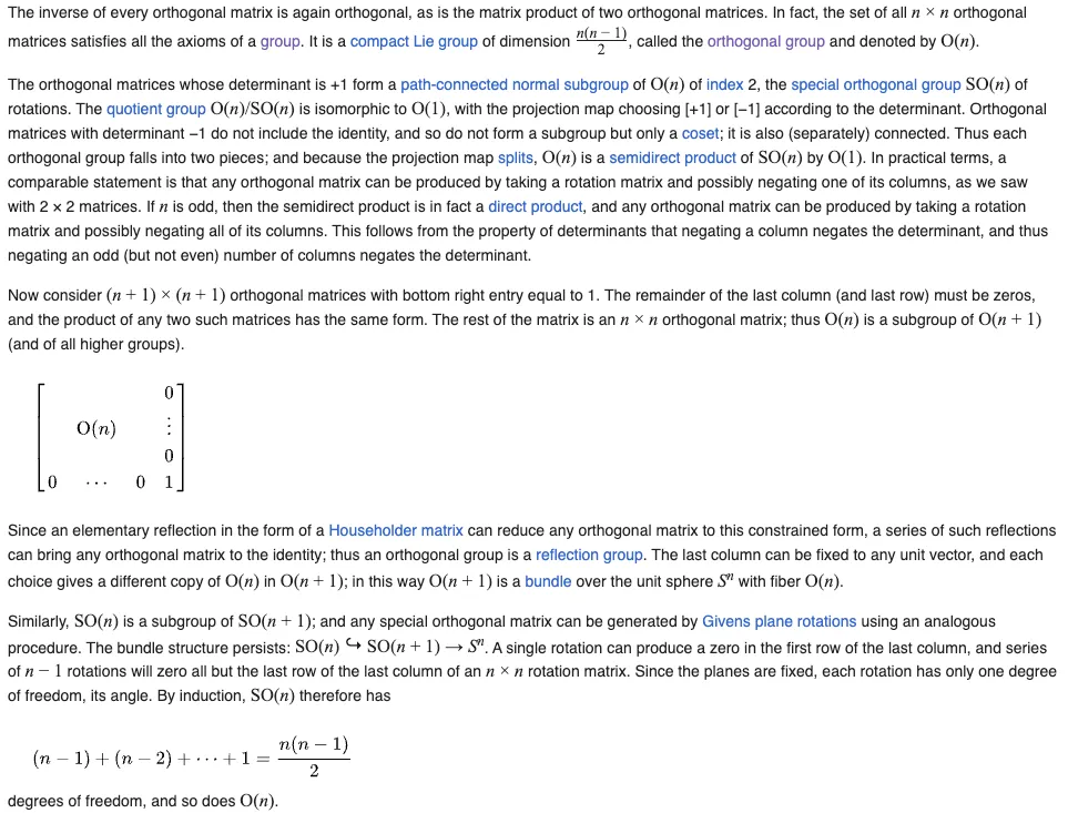I’d say my proof is cleaner, no? :P

$O(n)$ is not the same as $SO(n)$

I think my biggest mistake was assuming that all orthogonal matrices are rotation matrices. Wikipedia has a great explanation why you can’t have that conclusion on the orthogonal group page.

The orthogonal group in dimension n has two connected components. The one that contains the identity element is a normal subgroup, called the special orthogonal group, and denoted $SO(n)$. It consists of all orthogonal matrices of determinant 1. This group is also called the rotation group…

… The other component consists of all orthogonal matrices of determinant −1. This component does not form a group, as the product of any two of its elements is of determinant 1, and therefore not an element of the component.

Determinant $-1$..? Oh shit! A reflection is not a rotation. If $\hat{\imath}$ starts to the left of $\hat{\jmath}$, it should remain to the left of $\hat{\jmath}$. However, there are orthogonal transformations that, although preserve magnitude, do not preserve relative orientation. This causes the signed area of the determinant to flip when $\hat{\imath}$ and $\hat{\jmath}$ change chirality. The group I was trying to derive was the subgroup $SO(n)$, but since I didn’t constrain the basis vectors to maintain the same relative orientation as the identity matrix, I derived $O(n)$.

This problem gets worse in higher dimensions, where inversions generalize reflections. There’s a great Wikipedia page that discusses improper rotations like rotoflections and rotoinversions, if you’re curious. It’s especially important to account for improper rotations in vectors describing physical systems since many of them, like magnetic moment and angular velocity, are invariant under inversion. Ahh!! Such a silly mistake.

Conclusion

Although simple, I think the norm equation is favorite equation at the moment for its elegance and geometric interpretation. Overall, I learned a lot about linear algebra from working on this problem, and feel much more satisfied with rotation matrices. I hope you learnt something from reading it too.